Accelerating LLM Inference with Speculative Decoding: Notes on Medusa

This post briefly introduces speculative decoding and records what I learned while studying the Medusa method.

Speculative Decoding

Speculative decoding uses a lightweight draft model to generate multiple tokens at once, then asks the original LLM to verify them.

Suppose we generate $k$ tokens at a time. The cost of the process is approximately

$cost = decoding_{draft} \times k + forward_{llm}$

I use forward rather than decoding for the verification stage because verification can exploit the parallelism of a forward pass, much like training does.

To obtain a speedup, we therefore need:

$m \times decoding_{llm} > decoding_{draft} \times k + forward_{llm}$

Here, $m$ is the number of tokens among the $k$ candidates that are ultimately accepted. In other words, generating those $m$ tokens directly with the large model must take longer than drafting and verifying the candidate sequence.

This exposes the two central challenges of speculative decoding:

• Reduce the overhead.
• Increase the verification acceptance rate.

The key is therefore to find a suitable draft model.

In general, a smaller draft model introduces less overhead but produces worse predictions, reducing the acceptance rate. A larger draft model may predict more accurately, but its overhead can erase the performance gain.

Finding the right draft model can consequently be expensive. A smaller model from the same family is often a sensible choice, but models that are already in the 7B/13B range may not have a substantially smaller family member. Pretraining a new small model is costly, and without access to the original model’s training distribution it is difficult to match its token probability distribution closely enough to achieve a high acceptance rate.

Moreover, basic speculative decoding samples at the token level: the draft model generates tokens, and the target model verifies them. The lightweight model’s limited accuracy directly constrains the draft-token acceptance rate.

---

Medusa

One of the largest difficulties in conventional speculative decoding is obtaining a separate small draft model.

An alternative is to reuse the original LLM’s weights and train a small set of additional parameters. These incremental parameters can be viewed as corrections built on top of the original model and can predict draft tokens. This is what Medusa does: it uses multiple LM heads to predict tokens at different future positions.

1. Pipeline

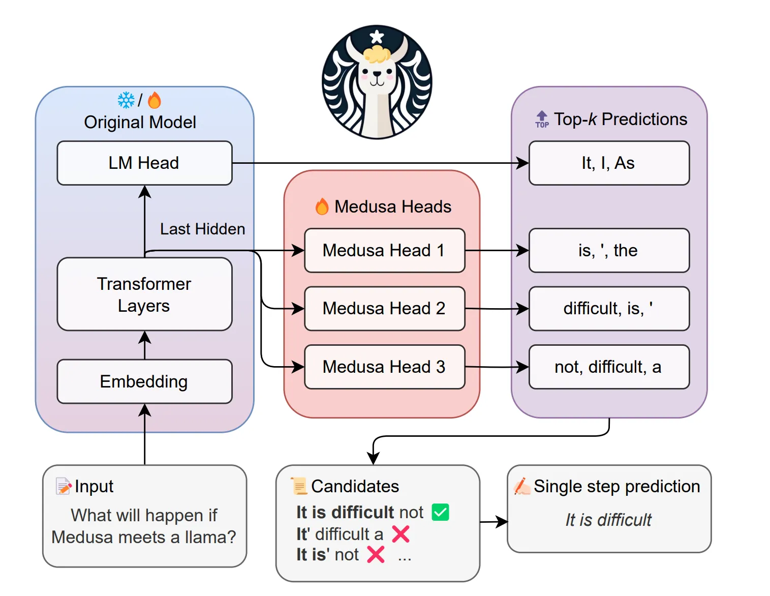
As shown above, different heads use the last hidden state to generate tokens for different future positions.

Define the next token as token $1$. At position $i$, the number of candidate tokens is a hyperparameter. The method selects the $top\text{-}s_i$ entries from that head’s logits, producing $s_i$ candidates. Together, these candidates form a tree.

The original LLM then verifies paths through this candidate tree and emits the accepted output.

2. Medusa Heads

Medusa uses a single-layer feed-forward network with a residual connection for each head:

$$p^{(k)}_t = \text{softmax} \left( W^{(k)}_2 \cdot \text{SiLU} \left( W^{(k)}_1 \cdot h_t \right) + h_t \right), \quad \text{where } W^{(k)}_2 \in \mathbb{R}^{d \times V}, \; W^{(k)}_1 \in \mathbb{R}^{d \times d}$$

Here, $p_t^{(k)}$ is the token distribution predicted by head $k$, while $p_t^{(0)}$ denotes the probability distribution produced by the model’s own LM head.

3. Tree Attention

Suppose a single speculative step generates candidates for the next $K$ positions. Because every position is predicted in parallel, the number of possible paths is the Cartesian product

$\prod_{i=1}^{K} s_i$

That is, a node at position $i$ may select any of the $s_{i+1}$ candidates at the next position as its child.

At depth $i$, the tree contains $\prod_{j=1}^{i} s_j$ nodes. A single speculative step must therefore verify $\prod_{i=1}^{K} s_i$ paths containing a total of

$\sum_{i=1}^{K} \prod_{j=1}^{i} s_j$

tokens. This grows explosively. With $K=4$ and $top\text{-}8$, there are 4,096 paths and 4,680 tokens in total.

Serial verification would require $\prod_{i=1}^{K} s_i$ forward passes before selecting the best path, which is far worse than the $K$ calls required by ordinary decoding. Medusa therefore needs a way to verify all paths in parallel.

The two-dimensional tree must be compressed into a one-dimensional sequence that still preserves the dependency relationships among nodes. Medusa accomplishes this with Tree Attention. Inspired by a causal mask, it applies a mask that prevents tokens on different paths from attending to one another.

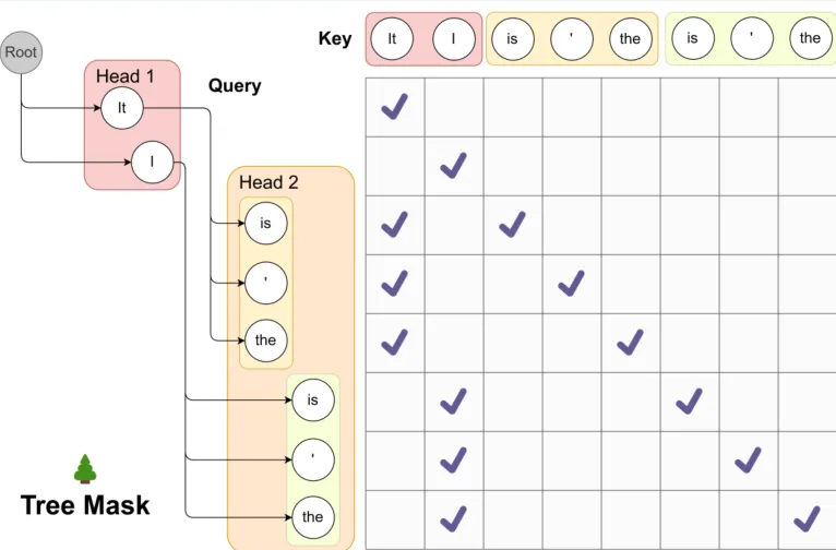
In the figure, checked cells indicate attention relationships that remain unmasked.

After computing $Q^{T}K$, we obtain a matrix whose rows and columns represent all candidate tokens. The attention output is a hidden_state tensor of size

$\left(\sum_{i=1}^{K} \prod_{j=1}^{i} s_j\right) \times hidden\text{-}dimension$

Passing these hidden states through the original LM head produces logit distributions. The LLM then applies its own sampling method, whether greedy decoding or sampling: the last hidden state passes through the LM head, softmax produces a probability distribution, and one token is sampled. Medusa checks whether this token exists among its first-level candidates. If it does, verification continues along the corresponding branch at the next level. This process repeats until it finds a valid path or reaches a level with no matching candidate.

4. Optimized Tree Construction

To reduce verification overhead, Medusa optimizes the verification sequence by pruning low-acceptance-probability paths from the draft tree in advance.

The paper uses a greedy algorithm. Given a fixed total number of tree nodes, it adds tokens one by one, always choosing the token with the largest contribution to the expected number of accepted tokens. The process is as follows:

1. Choose a calibration dataset and calculate the accuracy of the $i$-th ranked predicted token from head $k$. This should be empirical accuracy: the number of correct predictions divided by the total number of samples. Denote it by $a_k^{(i)}$.

2. After obtaining each node’s accuracy, assume that these accuracies are independent. For a path composed of candidates $[i_1,i_2,\ldots,i_k]$, the estimated path probability is the product $\prod_{j=1}^{k}a_j^{i_j}$.

3. Define a set $I$ whose elements correspond to every node in the tree, not only its leaves. Each element is the path $[i_1,i_2,\ldots,i_m]$ leading to that node. If the node is at depth $m$ and the total number of accepted tokens is $L$, then

$P(L \geq m)=\sum_{[i_1,i_2,\ldots,i_m]\in I}\prod_{j=1}^{m}a_j^{i_j}$

4. The expected number of accepted tokens is

$E[L]=\sum_{i=1}^{K}P(L\geq i)=\sum_{[i_1,i_2,\ldots,i_k]\in I}\prod_{j=1}^{k}a_j^{i_j}, \quad k \in [1,2,\ldots,K]$

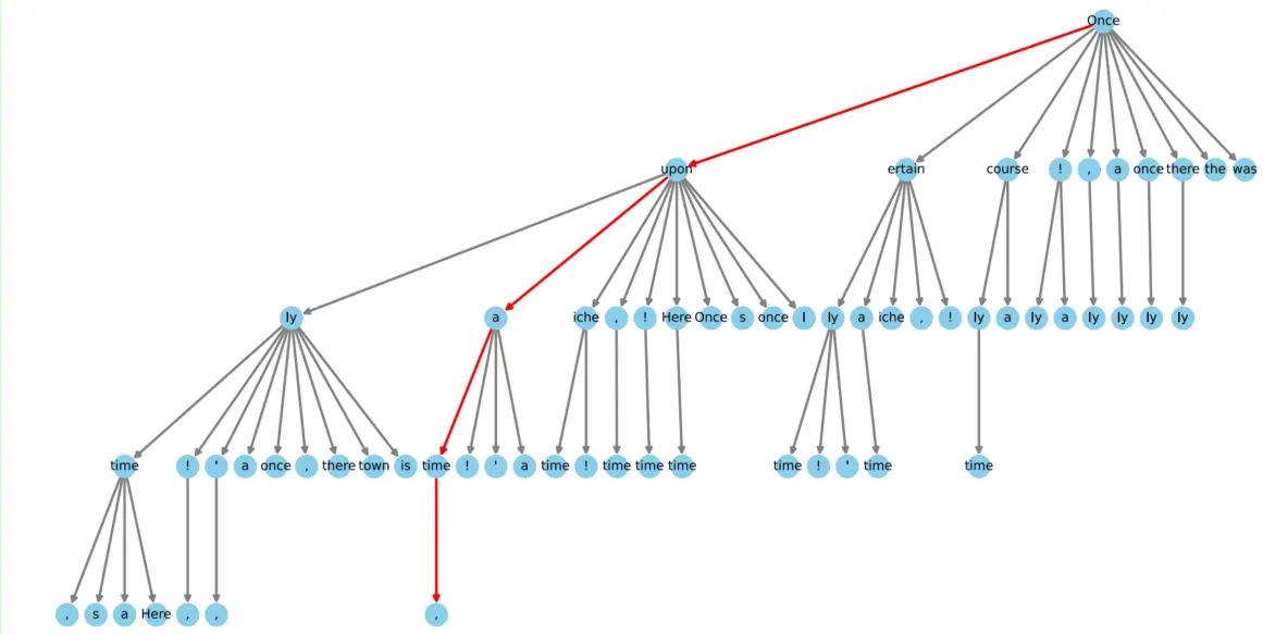
With the node count fixed, maximizing the expectation means selecting high-accuracy nodes. The resulting pruning procedure can produce a 64-node sparse tree like the one below.

5. Training

The paper reports that tuning the LLM alongside the Medusa heads performs better than training the heads alone.

1) Training the Heads Alone (Frozen Backbone)

The loss is computed with cross-entropy:

$\mathcal{L}_{k} = - \log p_t^{k}(y_{t+k+1})$

Here, $p_t^{k}(y)$ is the probability that head $k$ assigns to the correct token $y$.

As $k$ increases, $\mathcal{L}_{k}$ also tends to increase. Because all heads generate in parallel, tokens farther into the future are harder to predict. Medusa therefore introduces an additional weight $\lambda_k$ to balance the loss across heads:

$\mathcal{L}_{MEDUSA-1} = \sum_{k=1}^{K} - \lambda_{k} \log p_t^{(k)}(y_{t+k+1})$

The paper uses $0.8^k$ for $\lambda_k$.

2) Joint Training

• Combined loss: Add the LLM loss and introduce a weight $\lambda_0$ to balance it against the Medusa loss:

  $\mathcal{L}_{MEDUSA-2} = \mathcal{L}_{LM} + \lambda_{0} \mathcal{L}_{MEDUSA-1}$

• Different learning rates: Because the LLM is already trained, its learning rate should be much smaller than the learning rate used for the heads.

• Head warm-up: The heads have a large loss at the beginning of training. Training them alone for a short warm-up period prevents their large gradients from disrupting backpropagation through the LLM.

6. Summary

Medusa is a highly practical method. Its heads are extremely lightweight, yet they can produce a meaningful speedup.

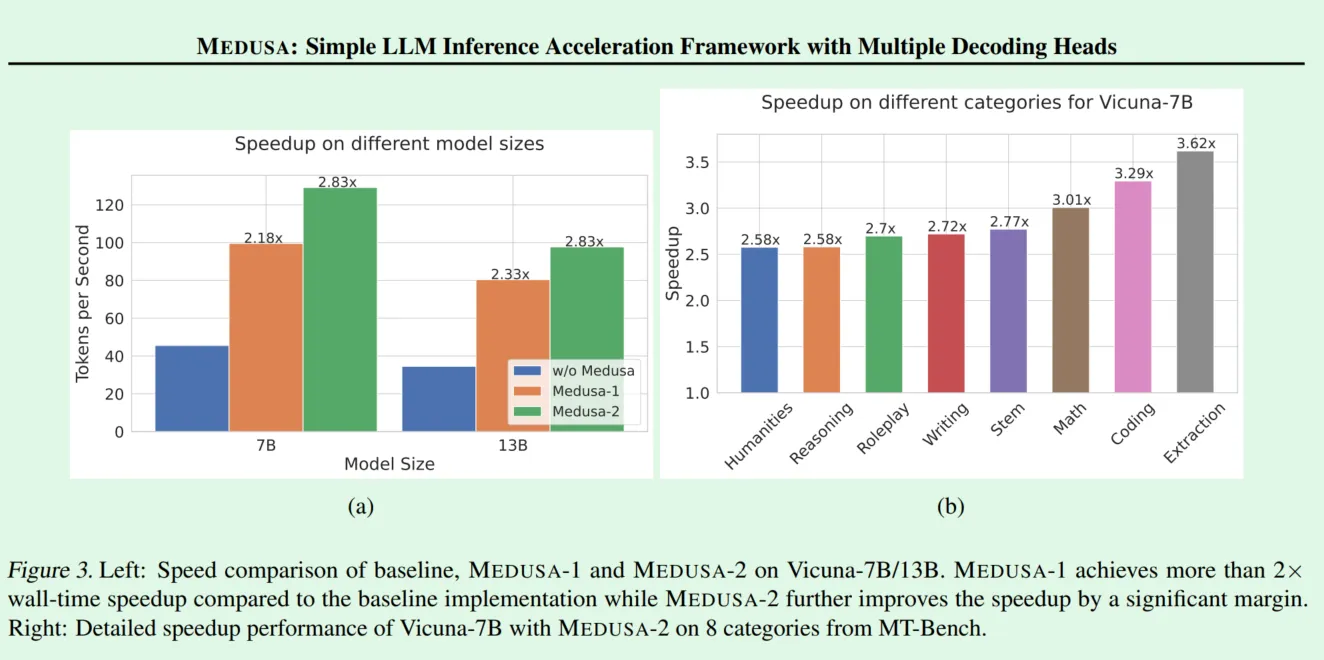
The draft tokens are still generated in parallel and cannot use information from earlier drafted tokens. I therefore expect its acceptance rate to be lower than that of EAGLE, which I plan to study next.