Learning the PyTorch Framework

Whenever I used PyTorch, I relied on LLM-generated code. I only knew how to add a few functional layers to an nn module and call the provided loss functions.

Now that I have time, I want to understand it more deeply.

Important Elements of PyTorch

1. Tensor

A tensor is a container representing a point or vector in a multidimensional space.

The progression is scalar → vector → matrix → tensor.

2.Autograd N Dynamic Computation Graph

PyTorch’s defining feature is automatic differentiation. While executing the forward pass, it records a dynamic computation graph, effectively constructing and destroying a DAG in real time.

You only need to pass requires_grad = true when initializing a tensor.

Advantages of a dynamic computation graph include:

• Greater flexibility, especially for conditionals and recursion.
• Easier debugging and modification, with direct access to intermediate results.

3. nn.Module

The neural network module encapsulates complex operations and integrates with the torch.optim optimizers.

Think of a large black box—the complete ResNet—containing many medium-sized black boxes—residual blocks—which themselves contain smaller boxes such as Conv2d and ReLU.

There are two ways to define a model: a custom class or nn.Sequential.

Feature	Custom class (inherits nn.Module)	nn.Sequential
forward definition	Must be defined manually	Runs layers in sequence automatically
Flexibility	High; supports arbitrary complex logic	Low; supports simple sequential structures only
Best suited for	Complex networks, branches, and skip connections	Simple sequential networks and rapid prototypes

Sequential

No new class is required; simply compose layers in order.

model = nn.Sequential(
    nn.Conv2d(3, 32, 3),
    nn.ReLU(),
    nn.Conv2d(32, 64, 3),
    nn.ReLU(),
    nn.Flatten(),
    nn.Linear(64 * 26 * 26, 10)
)

Custom Class

Subclass nn.Module, define the network layers in __init__, and define the data flow in forward.

Workflow

1. Objective (loss function): Define the distance between the “ideal state” and the current state.

2. Perception (forward): The system evaluates the input using its current parameters.

3. Feedback (backward): After recognizing the error, the system uses calculus to determine the direction of gradient descent.

4. Correction (optimizer): Adjust the parameters based on that feedback.

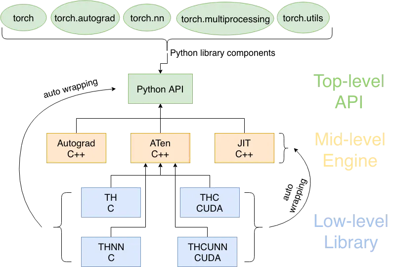
PyTorch Architecture

The following diagram summarizes the architecture:

┌─────────────────────────────────────────────────────────────┐
│                    PyTorch Ecosystem                         │
├─────────────────────────────────────────────────────────────┤
│  torchvision  │  torchtext  │  torchaudio  │ Specialist libs │
├─────────────────────────────────────────────────────────────┤
│                       PyTorch Core                           │
├───────────────┬─────────────────┬───────────────────────────┤
│   torch.nn    │   torch.optim   │      torch.utils          │
│ (neural nets) │ (optimizers)    │       (utilities)          │
├───────────────┼─────────────────┼───────────────────────────┤
│               │                 │   torch.utils.data        │
│  torch core  │  autograd        │      (data loading)        │
│  (tensors)   │  (autodiff)      │                            │
└───────────────┴─────────────────┴───────────────────────────┘